Deriving relative sea-level curves from the output of glacial isostatic adjustment models
Author
Isak Roalkvam
Published
February 10, 2026
This post provides a very brief introduction to physics-based models of glacial isostatic adjustment (GIA) and then goes on to show how the data derived from these can be accessed and used to retrieve a time-series of relative sea-level (RSL) change for a specific location. For this post I had to familiarise myself a bit more with the NetCDF format, which is popular for disseminating predictions from these kinds of models. The post is therefore meant to be a write-up with technical details for how to retrieve RSL data from the published result of GIA models, specifically ICE-7G_NA (Roy and Peltier 2015, 2017, 2018), along with some useful references. The technical walk-through in the text is done with Python, and at the end I have included a condensed version of the same workflow in R. I will underscore that I’m an archaeologist and not a geologist nor a geophysicists and I would encourage any reader (including future me) to approach this very much as a starting point for any dealings with GIA models.
1 Introduction to GIA models
A central aspect of my postdoc project pertains to investigating the relationship between archaeological sites and past sea-level change. I’m therefore in the process of getting a better grasp of the mechanisms that drive sea-level change and the ways in which this can be drawn on to reconstruct past sea-levels. My work with sea-level change has so far been based on empirical data and the shoreline displacement curves that have been derived from these (Roalkvam 2023, Romundset et al. 2026). These map changes in the relative sea-level over time. That is, they concern changes to the elevation of the sea relative to land. However, the relative sea-level is (predominantly) the result of two combined effects. The first is eustatic changes to the global mean sea-level resulting from exchange of water between ice sheets and ocean. The other is isostatic changes to the surface elevation of the Earth following from its response to the redistribution of weight caused by melting and forming ice sheets. An important endeavour within the field of geophysics and geodynamics is to combine physics-based models with data on ice history and Earth rheology in so-called GIA models to predict how the sea-level and surface elevation respond to changing ice loads over time, thereby making it possible to isolate the distinct effects of eustatic and isostatic adjustments (see e.g. Peltier 1998 for a fairly accessible account).
To be able to unpick the relationship between sea-level change as induced by forming or melting ice sheets that impact the global mean sea-level, and the adjustments to the surface of the Earth that follow from its viscoelsatic response to the redistribution of weight, these models are based on global histories of glaciation histories, although they might be focused towards specific regions. Despite being global in scope they can nonetheless be very valuable in conjunction with empirically based local reconstructions of sea-level change. For my purposes, this especially pertains to how empirically derived displacement curves are often based on fragmented data associated with considerable temporal as well as spatial uncertainties, meaning that the GIA models can provide an important frame of reference against which to evaluate or condition purely empirical reconstructions. As GIA models provide a model for glaciation history that is physically coherent given the global history of glacaiation and deglacation, any local deviation from these expected patterns can potentially offer valuable information on local conditions. Ultimately, GIA models can only be approximations of a complex real world system, but if properly validated against geomorphological records of past conditions they hold the potential to provide plausible estimates for future geodynamical change.
2 GIA-models and ICE-7G_NA (VM7)
The precise model output that I will work with here comes from ICE-7G_NA (VM7). This, along with the result from other variations of the ICE-xG models is available from the website of W.R. Peltier: https://www.atmosp.physics.utoronto.ca/~peltier/data.php.
To briefly present the core components of this model, the “ICE-7G” part of the name of the model refers to a specific ice thickness history. The extension “NA” refers to the fact that this model has been fine-tuned against geophysical observations in North America and then been evaluated in terms of its global exportability (see Roy and Peltier 2018). The parenthesis after the name of the ice history model refers to this data having been derived when employing the radial viscosity profile named VM7.
I will not attempt to lay out further details of how these models are calculated here, but in addition to the references given above, some important literature are the first formulations of the so-called sea-level equation (Farrell and Clark 1976; Clark et al. 1978) which forms the numerical foundation for GIA models, and a series of important refinements and further developments of the sea-level equation underlie current GIA models (see e.g. Peltier and Tushingham 1989; Mitrovica and Milne 2003; and Whitehouse 2018 for a historical account). In addition to these references, papers related to the previous versions of the iCE-xG models are also useful (e.g. Peltier et al. 2015, 2018; Purcell et al. 2016), in addition to those associated with other GIA models (e.g. Lambeck et al. 2014, 2017). Finally, while this post only deals with using existing results from a GIA model to plot RSL-change, open software is available to implement these models, allowing for the exploration of different input variables and parameter settings, and to adjust temporal and spatial resolutions (Spada and Melini 2019).
Returning to the GIA model we are dealing with here, the files representing the output from ICE-7G_NA (VM7) number a total of 48 NetCDF-files. They are named following the structure “I7G_NA.VM7_1deg.26.nc”, “I7G_NA.VM7_1deg.25.nc”, etc. You will notice that only the number just before “.nc” is changing between these. In these file names “I7G_NA.VM7” denotes the ice history and radial viscosity used in the model that produced the files. The part that reads “1deg” signifies that the data comes at a spatial resolution of 1x1 degrees. The number after this denotes the time-slice that a specific file pertains to, given in thousand years (ka) BP. In the examples above 26 and 25 ka BP, respectively. Finally, “nc” is the file extension for the NetCDF (Network Common Data Form) format.
3 NetCDF and xarray in Python
To precisely recreate the steps and output to follow, you will need to download the ICE-7G_NA files from Peltier’s website linked to above. In total, these have a size of about 38 MB. However, the code will also run with a smaller subset of the files if you only want to explore some of the functionality of the code. As stated in the beginning, I will work through this in Python in some detail, but a condensed version to achieve the same in R can be found towards the end. To read in NetCDF data in Python we can use the xarray library (Hoyer and Hamman 2017). We’ll start by reading in and exploring one of these files. I’ve chosen the one pertaining to 12 ka BP for this:
import osimport xarray as xr# Replace file path to where you have stored your NetCDF file(s) to load the datads = xr.open_dataset("../../../ICE-7G_NA(VM7)/I7G_NA.VM7_1deg.12.nc")# Print the structure of the xarray datasetprint(ds)
<xarray.Dataset> Size: 782kB
Dimensions:    (lat: 180, lon: 360)
Coordinates:
  * lat        (lat) float64 1kB -89.5 -88.5 -87.5 -86.5 ... 86.5 87.5 88.5 89.5
  * lon        (lon) float64 3kB 0.5 1.5 2.5 3.5 4.5 ... 356.5 357.5 358.5 359.5
Data variables:
    stgit      (lat, lon) float32 259kB ...
    Topo       (lat, lon) float32 259kB ...
    Topo_Diff  (lat, lon) float32 259kB ...
Attributes:
    Model:            ICE=ICE-7G_NA, Viscosity=VM7
    Date:             December 17, 2019
    Author:           W.R. Peltier, Dept of Physics, Univ of Toronto,Canada
    Acknowledgement:  Please cite following papers [PAPER1 and PAPER2 investi...
    PAPER1:           Roy, Keven, and W. R. Peltier - Glacial isostatic adjus...
    PAPER2:           Roy, Keven, and W. R. Peltier - Space-geodetic and wate...
    PAPER3:           Roy, Keven, and W. R. Peltier - Relative sea level in t...
This tells us that the data has two coordinates given in latitude (lat) and longitude (lon), and three data variables, the values of which are mapped to these coordinates. At the bottom we also get some metadata associated with the file. The first of the three data variables is ice thickness (stgit). That is, the values for stgit for a given coordinate pair gives the thickness of ice cover at that location at 12 ka BP. The second variable gives the topography (Topo), which is the surface elevation of land, ocean bottom (bathymetry) and ice cover, with 0 m representing the present-day mean sea-level. The final variable is the difference between the topography at this time slice and the present topography (Topo_Diff). To find the relative sea-level for a given location we will use the Topo_Diff variable.
Where ice is present the difference to the present surface elevation will be defined by the thickness of the ice and not the sea. So for locations covered by ice the RSL is undefined. In other areas where Topo_Diff is positive this indicates that the surface was higher than what it was at 12 ka BP, meaning that the relative sea-level was lower. Conversely, negative values for Topo_Diff indicates that the surface was lower in the past, and consequently that the RSL was higher. This therefore means that by flipping the sign of Topo_Diff we effectively find the relative sea-level for any given location, provided it was not covered by ice at that point in time. (Note that the output of other GIA models might look different from this, and sometimes already hold a variable for RSL).
# Change the sign of Topo_Diff and exclude areas covered by icersl =-ds["Topo_Diff"].where(ds["stgit"] ==0)
4 Global map of ice cover and RSL at 12 ka BP
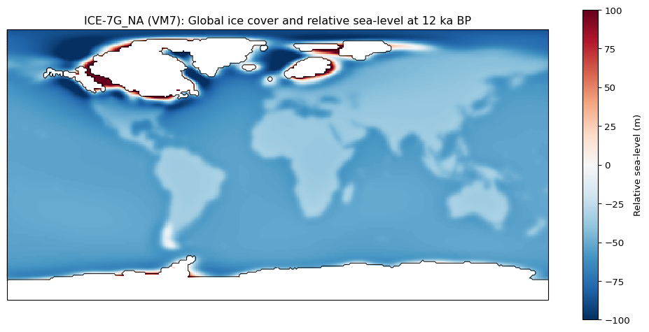
As both a sanity check and to see what the global pattern for ice cover and relative sea-level looks like according to ICE-7G_NA at 12 ka BP we can plot this on a map:
# Import libraries for plotting and handling coordinate reference systemsimport matplotlib.pyplot as pltfrom matplotlib.colors import TwoSlopeNormimport cartopy.crs as ccrsimport cartopy.feature as cfeature# Set up plotfig = plt.figure(figsize = (13, 6))# Provide a coordinate reference system that is often used with global dataax = plt.axes(projection = ccrs.PlateCarree())# Ice cover and relative sea levelpcm = plt.pcolormesh(ds.lon, ds.lat, rsl, shading ="auto", cmap ="RdBu_r",# Center the colour scale and limit its range to +/- 100 m norm = TwoSlopeNorm(vmin =-100, vcenter =0, vmax =100))# Plot the outline of the ice coversax.contour(ds.lon, ds.lat, ds.stgit, levels = [0], colors ="black", linewidths =0.7)# Plot labels and titleplt.colorbar(pcm, label ="Relative sea-level (m)")plt.xlabel("Longitude")plt.ylabel("Latitude")plt.title("ICE-7G_NA (VM7): Global ice cover and relative sea-level at 12 ka BP");
This looks sensible. Areas closer to glaciated areas tend to have a higher RSL relative to the present, and areas further afield have a smaller or negative RSL. We can now use all of the NetCDF files to find the GIA predicted trajectory for RSL change over time at some specific locations.
5 RSL-change for specific locations
As my postdoc project deals with the region of Kattegat and Skagerrak, I will choose locations from this area, but you can replace the coordinates in the code below to whatever location you are interested in.
First we will need to read in all of the NetCDF files to be able to combine the RSLs for each time-slice into a time-series. This could be done by a for-loop that reads in each individual file and extracts the time and RSL at the location of interest. For a bit more stability and functionality, and to make it easier to extract RSL-change for other locations later on, we will instead read in the NetCDF files and combine these in a xarray stack and assign each element a time coordinate to help us keep track of them.
# Import some additional libraries to facilitate reading in multiple files and# manipulating theseimport reimport osimport numpy as np# As above, replace this file path to where you have stored your NetCDF filespath ="../../../ICE-7G_NA(VM7)"# Get a list all the files in the directoryfiles = os.listdir(path)# Exlude anything but the NetCDF files # (just in case some temporary files or similar are in there)files_nc = [i for i in files if i.endswith('.nc')]# Define a regex function to find the time assigned to each file, which# falls between the string elements "1deg." and ".nc"def get_agebp(file):return(float(re.search(r'1deg.(.*?).nc', file).group(1)))# Get age ka BP for each file, sort these from oldest to youngest and store them# so that they can be assigned to the data when it has been loadedtimes_ka =sorted(np.array([get_agebp(f) for f in files_nc]), reverse =True)# Use the function again to get a list of file names sorted from oldest to youngestfiles_sorted =sorted(files_nc, key = get_agebp, reverse =True)# Append the full path to these chronologically sorted file namesfiles_full = [os.path.join(path, name) for name in files_sorted]# Read in files in a single xarray stack with a time dimensionds = xr.open_mfdataset( files_full, combine ="nested", concat_dim ="time") # The time dimension is currently just an index going from 0-48, so here we'll assign # the actual ages ka BP.ds = ds.assign_coords(time = times_ka)ds["time"].attrs["units"] ="ka BP"ds["time"].attrs["long_name"] ="Model age"# Print the structure of the dataprint(ds)
<xarray.Dataset> Size: 37MB
Dimensions:    (time: 48, lat: 180, lon: 360)
Coordinates:
  * time       (time) float64 384B 26.0 25.0 24.0 23.0 22.0 ... 1.5 1.0 0.5 0.0
  * lat        (lat) float64 1kB -89.5 -88.5 -87.5 -86.5 ... 86.5 87.5 88.5 89.5
  * lon        (lon) float64 3kB 0.5 1.5 2.5 3.5 4.5 ... 356.5 357.5 358.5 359.5
Data variables:
    stgit      (time, lat, lon) float32 12MB dask.array<chunksize=(1, 180, 360), meta=np.ndarray>
    Topo       (time, lat, lon) float32 12MB dask.array<chunksize=(1, 180, 360), meta=np.ndarray>
    Topo_Diff  (time, lat, lon) float32 12MB dask.array<chunksize=(1, 180, 360), meta=np.ndarray>
Attributes:
    Model:            ICE=ICE-7G_NA, Viscosity=VM7
    Date:             December 17, 2019
    Author:           W.R. Peltier, Dept of Physics, Univ of Toronto,Canada
    Acknowledgement:  Please cite following papers [PAPER1 and PAPER2 investi...
    PAPER1:           Roy, Keven, and W. R. Peltier - Glacial isostatic adjus...
    PAPER2:           Roy, Keven, and W. R. Peltier - Space-geodetic and wate...
    PAPER3:           Roy, Keven, and W. R. Peltier - Relative sea level in t...
You can see that time is now a third dimension and that this has 48 unique values, representing the 48 NetCDF files and their corresponding time-slice ages.
5.1 Regional map of Fennoscandia
Before extracting the RSL for some chosen locations in the Kattegat-Skagerrak area, we can create a map that uses data from multiple of the time slices and plots out the location of the points for where we’ll extract RSL curves. I’ve chosen Oslo, Göteborg and Aarhus for this. An important note to make here is that I’ve found the coordinates based on a coordinate system (WGS84, EPSG:4327) with a convention for longitude going from -180 to 180 whereas ICE-7G_NA uses a convention where longitude goes from 0 to 360. With positive values for longitude this has no consequence, but if the longitudinal values were negative they would have to be translated by using the modulo operator. (I’ve included this for the longitudinal values below to show how this can be done although it has no effect here as all the values for longitude are positive).
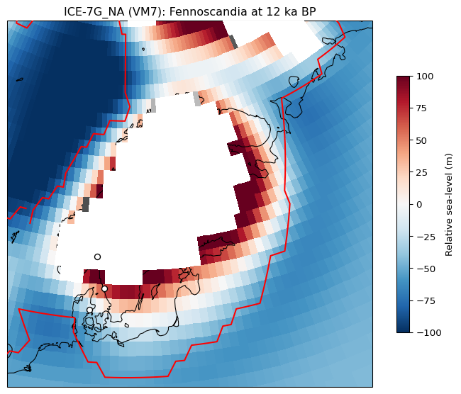
# Coordinates for Oslo, Göteborg and Aarhusosl_lat =59.90osl_lon =10.75%360gbg_lat =57.70gbg_lon =11.97%360aar_lat =56.14aar_lon =10.20%360# Time-slices to plotds_12ka = ds.sel(time =12)ds_lgm = ds.sel(time =21) # LGM at approx. 21 ka BP# RSL where there is not ice at 12 ka BPrsl_12ka =-ds_12ka["Topo_Diff"].where(ds_12ka["stgit"] ==0)# Mask layer to colour ice whiteice_12ka = ds_12ka["stgit"].where(ds_12ka["stgit"] >0)# Projection for Fennoscandiaproj = ccrs.LambertConformal(central_longitude =15, central_latitude =62, standard_parallels = (55, 70))# Set up plot with projectionfig = plt.figure(figsize = (9, 7))ax = plt.axes(projection = proj)# Set map extent to Fennoscandiaax.set_extent([2, 42, 50, 75], crs = ccrs.PlateCarree())# RSL layerpcm = ax.pcolormesh(ds.lon, ds.lat, rsl_12ka, transform = ccrs.PlateCarree(), cmap ="RdBu_r", norm = TwoSlopeNorm(vmin =-100, vcenter =0, vmax =100), shading ="auto", zorder =1)# Ice maskax.pcolormesh(ds.lon, ds.lat, ice_12ka, transform = ccrs.PlateCarree(), cmap ="gray", shading ="auto", vmin =0, vmax =1, zorder =3)# LGM ice cover outlineax.contour(ds.lon, ds.lat, ds_lgm["stgit"], levels = [0], colors="red", linewidths =1.5, transform = ccrs.PlateCarree(), zorder =4)# Add points for Oslo, Göteborg and Aarhusax.plot(osl_lon, osl_lat, marker="o", markersize =6, color ="white",markeredgecolor ="black", transform = ccrs.PlateCarree(), zorder =5)ax.plot(gbg_lon, gbg_lat, marker="o", markersize =6, color ="white",markeredgecolor ="black", transform = ccrs.PlateCarree(), zorder =6)ax.plot(aar_lon, aar_lat, marker="o", markersize =6, color ="white",markeredgecolor ="black", transform = ccrs.PlateCarree(), zorder =7)# Add coastline for areas not covered by iceax.coastlines(resolution="50m", linewidth =0.8, zorder =2)# RSL with colour gradient legendplt.colorbar(pcm, ax = ax, shrink =0.7, pad =0.05, label ="Relative sea-level (m)")# Titleax.set_title("ICE-7G_NA (VM7): Fennoscandia at 12 ka BP");
And here we have the resulting map showing RSL at 12 ka BP, areas covered by ice indicated in white, the outline of the ice cover at the Last Glacial Maximum (LGM) given in red, and the location of Oslo, Göteborg and Aarhus as points. We’ll now use the coordinates for the points to find RSL change over time at these locations.
5.2 RSL-change in Aarhus, Göteborg and Oslo
Now that we have the complete time-series of GIA model output in an xarray stack and point coordinates for Oslo, Göteborg and Aarhus we can derive the trajectory for RSL change at these locations. A point worth making here is that the results from the GIA model is provided as a grid and our point coordinates might fall at different positions within these grid cells. It is therefore appropriate to interpolate the value for each point location based on their position on the grid. Here I’ve done this simply using the nearest neighour method from xarray, but other approaches could also be been explored.
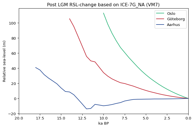
# Retrieve the data for the point representing Göteborg, using nearest neighbour# to interpolate the values to this point.point_gbg = ds.sel(lat = gbg_lat, lon = gbg_lon, method ="nearest")# Retrieve the RSL values by flipping the Topo_Diff sign and exclude periods when# Göteborg was covered by icersl_gbg =-point_gbg["Topo_Diff"].where(point_gbg["stgit"] ==0)# Transform this into a pandas series amenable for plottingrsl_gbg_ts = rsl_gbg.to_series()# Repeat for Oslopoint_osl = ds.sel(lat = osl_lat, lon = osl_lon, method ="nearest")rsl_osl =-point_osl["Topo_Diff"].where(point_osl["stgit"] ==0)rsl_osl_ts = rsl_osl.to_series()# Repeat for Aarhuspoint_aar = ds.sel(lat = aar_lat, lon = aar_lon, method ="nearest")rsl_aar =-point_aar["Topo_Diff"].where(point_aar["stgit"] ==0)rsl_aar_ts = rsl_aar.to_series()# Call to plotplt.figure(figsize=(8,5))plt.plot(point_osl["time"], rsl_osl_ts, color ='#27b376', label ='Oslo')plt.plot(point_gbg["time"], rsl_gbg_ts, color ='#bf212f', label ='Göteborg')plt.plot(point_osl["time"], rsl_aar_ts, color ='#264b96', label ='Aarhus')plt.legend()plt.xlabel("ka BP")plt.ylabel("Relative sea-level (m)")plt.title("Post LGM RSL-change based on ICE-7G_NA (VM7)")plt.gca().invert_xaxis() plt.xlim(20, 0);
It is worth highlighting that these curves do appear to deviate in some important ways from the local data on RSL change from these locations (see Rosentau et al. 2021; Romundset et al. 2026). In the area of Göteborg, for example, empirical data suggests the occurrence of a mid-Holocene sea-level transgression, which the GIA model does not indicate. This points to the value of the common exercise of comparing multiple GIA models and experimenting with their parameter settings when exploring RSL change in a given location, and to the value of also contrasting their output with empirical data. While GIA models can certainly be a valuable addition to the repertoire for archaeologists concerned with past sea-level change, a GIA model can hardly be assumed to directly provide reliable reconstruction for RSL change at a given location at the site-level scale that typically concern archaeologists.
6 Rough outline in R
NoteExpand to see condensed R code
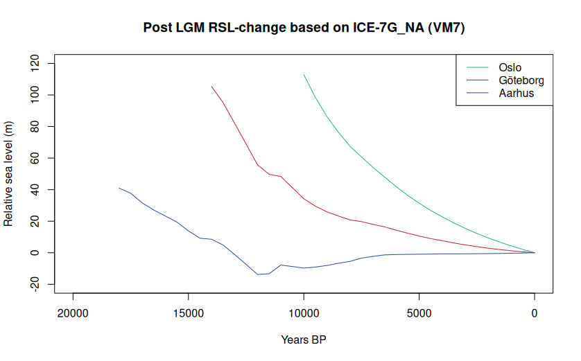
This R code gives a rough outline of how to you can achieve the same results as was achieved using Python above.
# Uncomment the lines below to install the packages used in the script# install.packages("terra")# install.packages("stringr")# install.packages("here")library(terra) # For handling NetCDF files and spatial datalibrary(stringr) # For wokring with strings when loading fileslibrary(here) # For file paths relative to the directory where the R script is located# Replace file path to where you have stored the NetCDF filesfiles <-list.files(path = here("../ICE-7G_NA(VM7)"), pattern ="\\.nc$", full.names = TRUE)# Get the age of the time-slice of each fileages_kBP <-as.numeric(str_extract(files, "(?<=1deg\\.)[0-9]+(\\.[0-9]+)?"))# Order the list of file names based on thisfiles_sorted <- files[order(ages_kBP, decreasing = TRUE)]# And get the sorted numbers to assign to a time dimension of the rasters in the stack.# Using the full age BP instead of ka BP, due to how terra handles the time dimensionages_kBP <- sort(ages_kBP, decreasing = TRUE) *1000# Read in the rasters as a stack and rotate() to change longitude convention from# going from 0 to 260 to -180 to 180topodiff_stack <- rotate(rast(files_sorted, subds ="Topo_Diff"))ice_stack <- rotate(rast(files_sorted, subds ="stgit"))# Assign ages to the stackstime(topodiff_stack) <- ages_kBPtime(ice_stack) <- ages_kBP# Retrieve RSL and ice cover at 12 ka BP for ploti_12ka <- which.min(abs(time(topodiff_stack) -12000))# RSL at 12 ka BPrsl_12ka <--topodiff_stack[[i_12ka]]# Ice cover at 12 ka BP, set to NA where ice is not presentice_12ka <- ice_stack[[i_12ka]]ice_12ka[ice_12ka <=0] <- NA# Point vector features for Oslo, Göteborg and Aarhusosl <- vect(data.frame(lon =10.75, lat =59.90), geom = c("lon", "lat"), crs ="EPSG:4326")gbg <- vect(data.frame(lon =11.97, lat =57.70), geom = c("lon", "lat"), crs ="EPSG:4326")aar <- vect(data.frame(lon =10.20, lat =56.14), geom = c("lon", "lat"), crs ="EPSG:4326")# Simple map plot for a sanity check (not reproduced here)plot(rsl_12ka, main ="ICE-7G_NA (VM7): RSL and ice cover at 12 ka BP")plot(ice_12ka, col ="white", legend = FALSE, add = TRUE)plot(osl, cex =0.5, add = TRUE)plot(gbg, cex =0.5, add = TRUE)plot(aar, cex =0.5, add = TRUE)# Flip sign of Topo_Diff and extract this for Oslo.# Remove the ID associated with the values using [1, -1]rsl_osl <- extract(-topodiff_stack, osl)[1, -1]# Extract ice cover for Osloice_osl <- extract(ice_stack, osl)[1, -1]# Remove RSL for when Oslo was covered by ice, as this is undefinedrsl_osl <-as.numeric(ifelse(ice_osl >0, NA, rsl_osl))# Repeat for Göteborgrsl_gbg <- extract(-topodiff_stack, gbg)[1, -1]ice_gbg <- extract(ice_stack, gbg)[1, -1]rsl_gbg <-as.numeric(ifelse(ice_gbg >0, NA, rsl_gbg))# Repeat for Aarhusrsl_aar <- extract(-topodiff_stack, aar)[1, -1]ice_aar <- extract(ice_stack, aar)[1, -1]rsl_aar <-as.numeric(ifelse(ice_aar >0, NA, rsl_aar))# Create data frames for plottingrsl_osl <- data.frame(BP = time(topodiff_stack), rsl = rsl_osl)rsl_gbg <- data.frame(BP = time(topodiff_stack), rsl = rsl_gbg)rsl_aar <- data.frame(BP = time(topodiff_stack), rsl = rsl_aar)# Call to plotplot(rsl_osl$BP, rsl_osl$rsl, type="n", xlim = c(20000, 0), ylim = c(-20, 120), xlab ="Years BP", ylab ="Relative sea level (m)", main ="Post LGM RSL-change based on ICE-7G_NA (VM7)")lines(rsl_osl$BP, rsl_osl$rsl, type="l", col ="#27b376")lines(rsl_gbg$BP, rsl_gbg$rsl, type="l", col ="#bf212f")lines(rsl_aar$BP, rsl_aar$rsl, type="l", col ="#264b96")legend("topright", legend = c("Oslo", "Göteborg", "Aarhus"), col = c("#27b376", "#bf212f", "#264b96"), lty =1)
7 References
Clark, J. A., W. E. Farrell, and W. R. Peltier. 1978. Global Changes in Postglacial Sea Level: A Numerical Calculation. Quaternary Research 9(3):265–287. https://doi.org/10.1016/0033-5894(78)90033-9.
Hoyer, S., and J. Hamman. 2017. Xarray: N-D Labeled Arrays and Datasets in Python. Journal of Open Research Software 5(1):10. https://doi.org/10.5334/jors.148.
Lambeck, K., H. Rouby, A. Purcell, Y. Sun, and M. Sambridge. 2014. Sea Level and Global Ice Volumes from the Last Glacial Maximum to the Holocene. Proceedings of the National Academy of Sciences 111(43):15296–15303. https://doi.org/doi:10.1073/pnas.1411762111.
Lambeck, Kurt, A. Purcell, and S. Zhao. 2017. North American Late Wisconsin Ice Sheet and Mantle Viscosity from Glacial Rebound Analyses. Quaternary Science Reviews 158:172–210. https://doi.org/10.1016/j.quascirev.2016.11.033.
Peltier, W. R. 1998. Postglacial Variations in the Level of the Sea: Implications for Climate Dynamics and Solid-Earth Geophysics. Reviews of Geophysics 36(4):603–689. https://doi.org/10.1029/98RG02638.
Peltier, W. R., D. F. Argus, and R. Drummond. 2015. Space Geodesy Constrains Ice Age Terminal Deglaciation: The Global ICE-6G_C (VM5a) Model. Journal of Geophysical Research: Solid Earth 120(1):450–487. https://doi.org/10.1002/2014JB011176.
Peltier, W. R., D. F. Argus, and R. Drummond. 2018. Comment on ‘An Assessment of the ICE-6G_C (VM5a) Glacial Isostatic Adjustment Model’ by Purcell et al. Journal of Geophysical Research: Solid Earth 123(2):2019–2028. https://doi.org/10.1002/2016JB013844.
Purcell, A., P. Tregoning, and A. Dehecq. 2016. An Assessment of the ICE6G_C(VM5a) Glacial Isostatic Adjustment Model. Journal of Geophysical Research: Solid Earth 121(5):3939–3950. https://doi.org/10.1002/2015JB012742.
Roalkvam, I. 2023. A Simulation-Based Assessment of the Relation between Stone Age Sites and Relative Sea-Level Change along the Norwegian Skagerrak Coast. Quaternary Science Reviews 299:107880. https://doi.org/10.1016/j.quascirev.2022.107880.
Romundset, A., I. Roalkvam, M. van Boeckel, F. Høgaas, K. E. Henningsmoen, H. I. Høeg, and R. Sørensen. 2026. Shoreline and Deglaciation Chronology in Southeast Norway. Boreas 55(1):29–56. https://doi.org/10.1111/bor.70024.
Rosentau, A., V. Klemann, O. Bennike, H. Steffen, J. Wehr, M. Latinović, M. Bagge, A. Ojala, M. Berglund, G. P. Becher, K. Schoning, A. Hansson, L. Nielsen, L. B. Clemmensen, M. U. Hede, A. Kroon, M. Pejrup, L. Sander, K. Stattegger, K. Schwarzer, R. Lampe, M. Lampe, S. Uścinowicz, A. Bitinas, I. Grudzinska, J. Vassiljev, T. Nirgi, Y. Kublitskiy, and D. Subetto. 2021. A Holocene Relative Sea-Level Database for the Baltic Sea. Quaternary Science Reviews 266:107071. https://doi.org/10.1016/j.quascirev.2021.107071.
Roy, K., and W. R. Peltier. 2015. Glacial Isostatic Adjustment, Relative Sea Level History and Mantle Viscosity: Reconciling Relative Sea Level Model Predictions for the US East Coast with Geological Constraints. Geophysical Journal International 201(2):1156–1181. https://doi.org/10.1093/gji/ggv066.
Roy, K., and W. R. Peltier. 2017. Space-Geodetic and Water Level Gauge Constraints on Continental Uplift and Tilting over North America: Regional Convergence of the ICE-6G_C (VM5a/VM6) Models. Geophysical Journal International 210(2):1115–1142. https://doi.org/10.1093/gji/ggx156.
Roy, K., and W. R. Peltier. 2018. Relative Sea Level in the Western Mediterranean Basin: A Regional Test of the ICE-7G_NA (VM7) Model and a Constraint on Late Holocene Antarctic Deglaciation. Quaternary Science Reviews 183:76–87. https://doi.org/10.1016/j.quascirev.2017.12.021
Spada, G., and D. Melini. 2019. SELEN4 (SELEN Version 4.0): A Fortran Program for Solving the Gravitationally and Topographically Self-Consistent Sea-Level Equation in Glacial Isostatic Adjustment Modeling. Geoscientific Model Development 12(12):5055–5075. https://doi.org/10.5194/gmd-12-5055-2019.
Whitehouse, P. L. 2018. Glacial Isostatic Adjustment Modelling: Historical Perspectives, Recent Advances, and Future Directions. Earth Surface Dynamics 6(2):401–429. https://doi.org/10.5194/esurf-6-401-2018.